Problem1 - b, c¶

Consider the case when \(H=W\) (a square cavity). Here, the Reynolds number, \(Re=UW/\nu\), characterizes the flow patters. Compute the steady state solutions for both \(Re=100\) and \(Re=500\). Plot the flow streamlines and centerline profiles (\(u\) vs. \(y\) and \(v\) vs. \(x\) through the center of the domain). For \(Re=100\), valdiate your method by comparing your results to data from given literature.

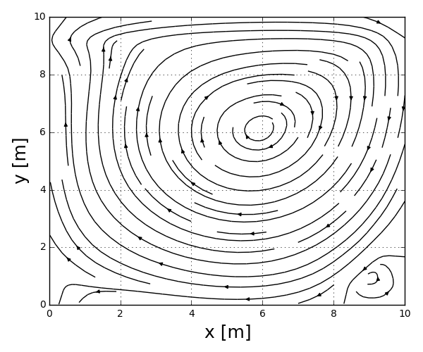
Re = 100¶

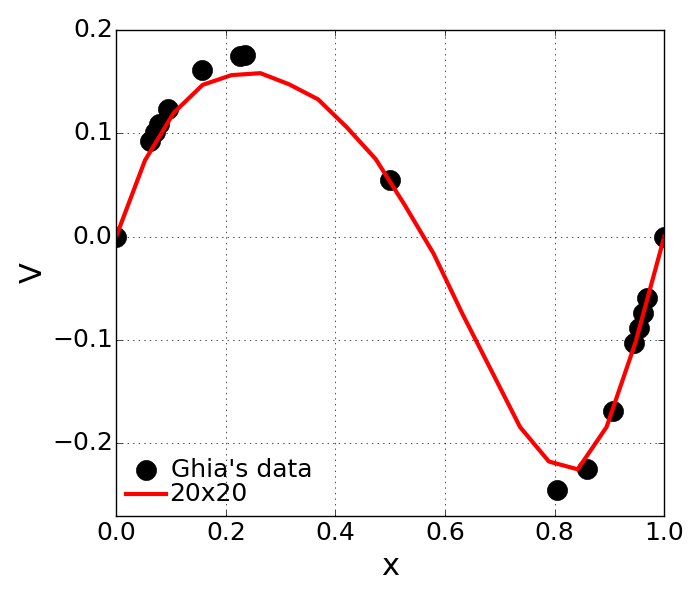
NxN = 20x20
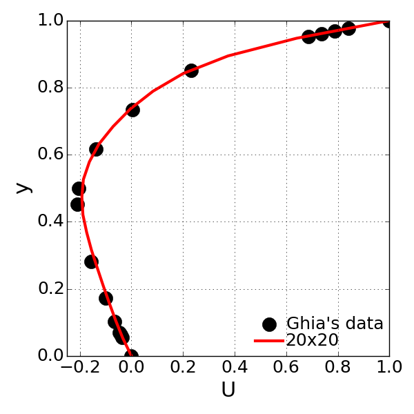
- u-velocity
- v-velocity
- Observation
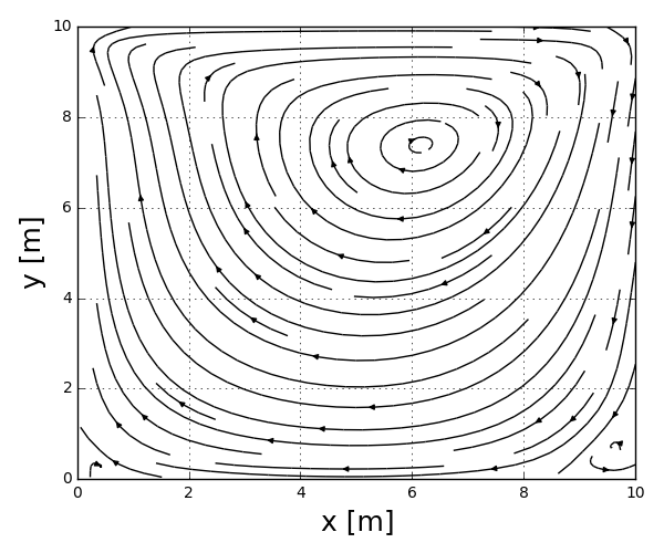
  - Streamlines roughly forms and recirculation zone in the bottom right can be found.
  - This course grid case shows bad estimation of u and v-velocity as compared to the Ghia’s data

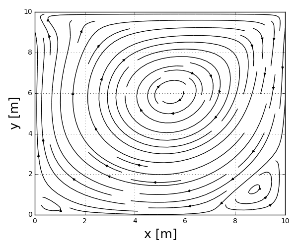
NxN = 40x40
- u-velocity
- v-velocity
- Observation
  - The predicted u- and v-velocity approached closer to the Ghia’s data

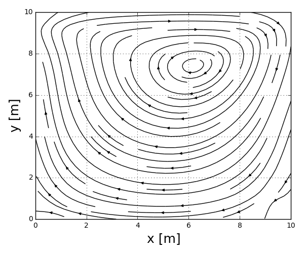
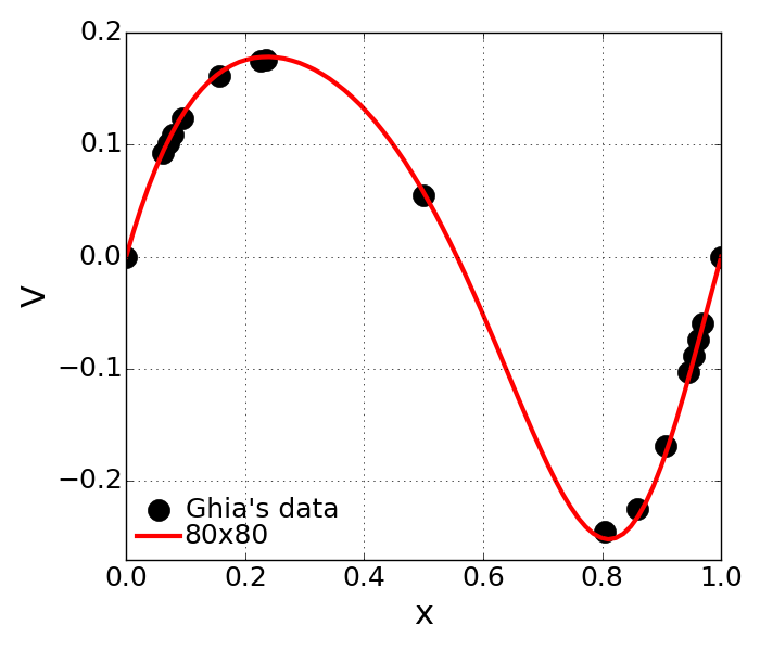
NxN = 80x80
- u-velocity
- v-velocity
- Observation
  - The currently predicted data seems to be almost identical with the Ghia’s solution.
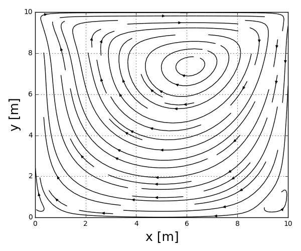
  - Recirculation zone in the bottom left and right seems more clear than the coarser grid cases.

Re = 500¶

NxN = 20x20

NxN = 80x80